
Type any function and see its shape straight away. Plot up to three at once in three colours to compare them, drag the trace point to read a value off a curve, and see where each one crosses zero.
—
KiwiBee uses optional Google Analytics, Google Ads, and Meta Pixel cookies to understand adult visitors, measure completed sign-ups, and improve campaigns. Essential cookies always stay on. OpenAI’s ChatGPT Ads Pixel also measures page views and completed enquiries after advertising consent, and may use hashed contact details for matching. Privacy policy
Monte Carlo & Buffon's Needle demonstrates how randomness can solve deterministic geometric problems. In Sphere in Cube (3D) mode, random points (x, y, z) rain into a cube of side 2R; because the inscribed sphere occupies exactly π/6 ≈ 52.36% of the cube's volume, multiplying the fraction of gold inside hits by 6 estimates π. Students can also switch to the classic 2D Circle in Square ratio (π/4) or Buffon's Needles, where sticks of length L dropped onto floorboards spaced D apart cross a line with probability 2L/(πD). Dragging the overhead emitter or firing 500-sample bursts drives the live convergence curve toward 3.14159 by the Law of Large Numbers.
A cube extending from −R to +R has side length 2R and volume (2R)³ = 8R³. A sphere of radius R inscribed inside it has volume (4/3)πR³. Dividing the sphere volume by the cube volume cancels R³ and gives (4/3)π / 8 = π / 6, so π = 6 × (V_sphere / V_cube).
In 1777 Georges-Louis Leclerc, Comte de Buffon showed that when a needle of length L (with L ≤ D) is dropped randomly onto parallel lines spaced D apart, the probability of crossing a line is P = 2L / (πD). Rearranging gives π ≈ 2L·N / (D·K).
Random sampling has standard error proportional to 1/√N. With only 50 darts, a few lucky or unlucky hits shift the ratio by several percent; reducing the error by a factor of 10 requires 100 times as many samples.
Monte Carlo simulations are essential in high-dimensional physics, radiation transport, financial risk modeling, computer graphics ray tracing, and AI tree search where exact integrals have too many dimensions to solve on a grid.
Drop it into your LMS, blog, or class site — free.
<iframe src="https://kiwibee.io/en/simulations/monte-carlo-probability-pi-3d-3d-simulation/embed" title="Monte Carlo & Buffon's Needle | KiwiBee" loading="lazy" allowfullscreen style="width:100%;height:min(70vh,620px);min-height:420px;border:0;border-radius:16px"></iframe>Continue exploring
Type any function and see its shape straight away. Plot up to three at once in three colours to compare them, drag the trace point to read a value off a curve, and see where each one crosses zero.

Spin a spinner, flip a coin or roll a die and watch two sets of bars: the chances the shapes predict, and the results you actually got. Ten spins prove nothing; a few hundred and the two are hard to tell apart.

Move m and watch the line tilt; move b and watch it slide. Or drag the two points on the line and read the equation it writes back. A rise-over-run staircase climbs the line so slope becomes something you can count.
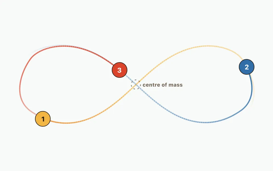
Compare a two-body orbit with three-body figure-eight motion, then add up to twelve bodies. Change initial masses, velocities and positions; watch orbit trails and numerical energy error.

Approximate the area under a curve with strips and choose how each takes its height: left edge, right edge, middle, or a sloping top. Push the strip count up and watch the error fall, with the running total plotted as its own curve.
From model to evidence
Use a worksheet to capture predictions, observations, and explanations after students explore.
KiwiBee's free teacher workspace brings lesson planning, worksheets, classroom tools, and gradebook together in one place.
Start free and create your first class Home
 All solutions
 Pricing
 About us
 KiwiBee for Non-profits
 Events & webinars
 For big organisations
 For schools
 For centers
 For team leaders
 For teachers
 AI and resources
 Resources
 Printable worksheets
 Lesson Packs
 Interactive simulations
 Teacher tools
 AI studio
 Ideas and research