
Type any function and see its shape straight away. Plot up to three at once in three colours to compare them, drag the trace point to read a value off a curve, and see where each one crosses zero.
—
KiwiBee uses optional Google Analytics, Google Ads, and Meta Pixel cookies to understand adult visitors, measure completed sign-ups, and improve campaigns. Essential cookies always stay on. OpenAI’s ChatGPT Ads Pixel also measures page views and completed enquiries after advertising consent, and may use hashed contact details for matching. Privacy policy
Linear Regression & Error Bowl connects statistics and optimization in a split 3D studio. On the left board, six draggable scatter points—including a high-leverage orange outlier—are fitted by a trial line y = mx + b. Attached to each point is a literal red square whose side equals the vertical residual |yᵢ − (mxᵢ + b)|, making its area equal to the squared error eᵢ². On the right stage, the total area of all squares is plotted as a 3D paraboloid bowl SSE(m, b) over slope and intercept parameter space. Students can drag the parameter marker across the bowl or toggle Snap to Optimal OLS to watch the marker settle into the unique global minimum (m̂, b̂) while monitoring r and R².
Squaring each vertical error eᵢ = yᵢ − ŷᵢ prevents positive errors above the line from canceling negative errors below the line, penalizes large misses heavily, and creates a smooth paraboloid bowl with a single unique minimum.
The two horizontal axes of the bowl are the trial slope m and trial intercept b, and the vertical height is the Sum of Squared Errors SSE(m, b). Every possible straight line corresponds to one point on that bowl, and the best-fit line sits at the lowest point.
Because errors are squared, a point twice as far from the line contributes four times as much to SSE. The regression line tilts strongly toward an outlier to keep that giant square from exploding in area.
Correlation r ranges from −1 to +1 and measures the direction and strength of a linear relationship. R² (the square of r in simple linear regression) ranges from 0% to 100% and tells what fraction of the variance in y is explained by x.
Drop it into your LMS, blog, or class site — free.
<iframe src="https://kiwibee.io/en/simulations/least-squares-linear-regression-3d-3d-simulation/embed" title="Linear Regression & Error Bowl | KiwiBee" loading="lazy" allowfullscreen style="width:100%;height:min(70vh,620px);min-height:420px;border:0;border-radius:16px"></iframe>Continue exploring
Type any function and see its shape straight away. Plot up to three at once in three colours to compare them, drag the trace point to read a value off a curve, and see where each one crosses zero.

Spin a spinner, flip a coin or roll a die and watch two sets of bars: the chances the shapes predict, and the results you actually got. Ten spins prove nothing; a few hundred and the two are hard to tell apart.

Move m and watch the line tilt; move b and watch it slide. Or drag the two points on the line and read the equation it writes back. A rise-over-run staircase climbs the line so slope becomes something you can count.
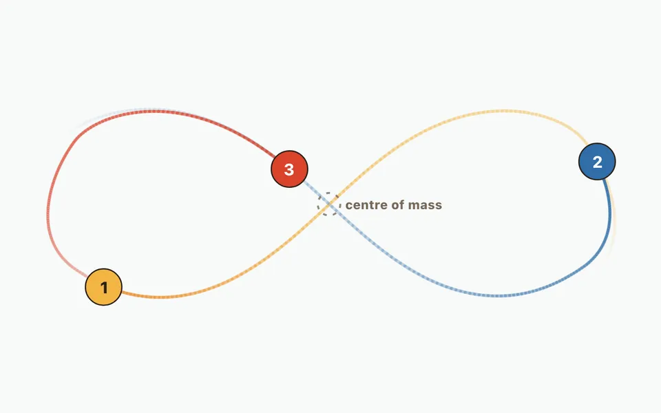
Compare a two-body orbit with three-body figure-eight motion, then add up to twelve bodies. Change initial masses, velocities and positions; watch orbit trails and numerical energy error.

Approximate the area under a curve with strips and choose how each takes its height: left edge, right edge, middle, or a sloping top. Push the strip count up and watch the error fall, with the running total plotted as its own curve.
From model to evidence
Use a worksheet to capture predictions, observations, and explanations after students explore.
KiwiBee's free teacher workspace brings lesson planning, worksheets, classroom tools, and gradebook together in one place.
Start free and create your first class Home
 All solutions
 Pricing
 About us
 KiwiBee for Non-profits
 Events & webinars
 For big organisations
 For schools
 For centers
 For team leaders
 For teachers
 AI and resources
 Resources
 Printable worksheets
 Lesson Packs
 Interactive simulations
 Teacher tools
 AI studio
 Ideas and research