
Digite qualquer função e veja o formato dela na hora. Trace até três de uma vez em três cores para compará-las, arraste o ponto de leitura para ler um valor da curva e veja onde cada uma cruza o zero.
—
O KiwiBee usa cookies opcionais do Google Analytics, Google Ads e Meta Pixel para entender os visitantes adultos, medir cadastros concluídos e melhorar as campanhas. Os cookies essenciais ficam sempre ativos. O Pixel de anúncios do ChatGPT da OpenAI também mede visitas e consultas enviadas após o consentimento publicitário e pode usar dados de contato com hash para correspondência. Política de privacidade
[Pt] Linear Regression & Error Bowl connects statistics and optimization in a split 3D studio. On the left board, six draggable scatter points—including a high-leverage orange outlier—are fitted by a trial line y = mx + b. Attached to each point is a literal red square whose side equals the vertical residual |yᵢ − (mxᵢ + b)|, making its area equal to the squared error eᵢ². On the right stage, the total area of all squares is plotted as a 3D paraboloid bowl SSE(m, b) over slope and intercept parameter space. Students can drag the parameter marker across the bowl or toggle Snap to Optimal OLS to watch the marker settle into the unique global minimum (m̂, b̂) while monitoring r and R².
[Pt] Squaring each vertical error eᵢ = yᵢ − ŷᵢ prevents positive errors above the line from canceling negative errors below the line, penalizes large misses heavily, and creates a smooth paraboloid bowl with a single unique minimum.
[Pt] The two horizontal axes of the bowl are the trial slope m and trial intercept b, and the vertical height is the Sum of Squared Errors SSE(m, b). Every possible straight line corresponds to one point on that bowl, and the best-fit line sits at the lowest point.
[Pt] Because errors are squared, a point twice as far from the line contributes four times as much to SSE. The regression line tilts strongly toward an outlier to keep that giant square from exploding in area.
[Pt] Correlation r ranges from −1 to +1 and measures the direction and strength of a linear relationship. R² (the square of r in simple linear regression) ranges from 0% to 100% and tells what fraction of the variance in y is explained by x.
Coloque no seu AVA, blog ou site da turma — de graça.
<iframe src="https://kiwibee.io/pt/simulations/least-squares-linear-regression-3d-3d-simulation/embed" title="Linear Regression & Error Bowl | KiwiBee" loading="lazy" allowfullscreen style="width:100%;height:min(70vh,620px);min-height:420px;border:0;border-radius:16px"></iframe>Continue explorando
Digite qualquer função e veja o formato dela na hora. Trace até três de uma vez em três cores para compará-las, arraste o ponto de leitura para ler um valor da curva e veja onde cada uma cruza o zero.

Gire uma roleta, jogue uma moeda ou role um dado e veja dois conjuntos de barras: as chances que os formatos preveem e os resultados que você realmente obteve. Dez giros não provam nada; com algumas centenas, os dois quase não se distinguem.

Mova m e veja a reta inclinar; mova b e veja a reta deslizar. Ou arraste os dois pontos da reta e leia a equação que ela devolve. Uma escada de “subida sobre avanço” sobe pela reta para que o coeficiente angular vire algo que dá para contar.
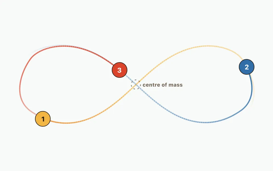
Compare uma órbita de dois corpos com o movimento em oito de três corpos e adicione até doze corpos. Altere massas, velocidades e posições iniciais; observe trajetórias e erro numérico de energia.

Aproxime a área sob uma curva com faixas e escolha como cada uma toma a altura: borda esquerda, borda direita, meio ou topo inclinado. Aumente o número de faixas e veja o erro cair, com a soma acumulada traçada como uma curva própria.
Do modelo ao registro
Use uma atividade para registrar previsões, observações e explicações depois que os alunos explorarem.
O espaço gratuito do professor da KiwiBee reúne em um só lugar o planejamento de aulas, as atividades, as ferramentas de sala e o diário de classe.
Comece grátis e crie sua primeira turma Início
 Todas as soluções
 Preços
 Sobre nós
 KiwiBee para organizações sem fins lucrativos
 Eventos e webinars
 Para grandes redes de ensino
 Para escolas
 Para centros educacionais
 Para líderes de equipe
 Para professores
 IA e recursos
 Recursos
 Atividades para imprimir
 Pacotes de aula
 Simulações interativas
 Ferramentas para professores
 Estúdio de IA
 Ideias e pesquisa